Rethink2m1

Aufgabe

This question is taken from McElreath, R. (2020). Statistical rethinking: A Bayesian course with examples in R and Stan (2. Ed.). Taylor and Francis, CRC Press.

2M1. Recall the globe tossing model from the chapter. Compute and plot the grid approximate posterior distribution for each of the following sets of observations. In each case, assume a uniform prior for p.

1. WWW
2. WWWL
3. LWWLWWW

Lösung

The solution is taken from this source.

library(tidyverse)

dist <- 
  tibble(
    # Gridwerte bestimmen:
    p_grid = seq(from = 0, to = 1, length.out = 20),
    # Priori-Wskt bestimmen:
    prior = rep(1, times = 20)) %>%
  mutate(
    # Likelihood berechnen:
    likelihood_1 = dbinom(3, size = 3, prob = p_grid),  # WWW
    likelihood_2 = dbinom(3, size = 4, prob = p_grid),  # WWWL
    likelihood_3 = dbinom(5, size = 7, prob = p_grid),  # LWWLWWW
    # unstand. Posterior-Wskt:
    unstand_post_1 = likelihood_1 * prior,
    unstand_post_2 = likelihood_2 * prior,
    unstand_post_3 = likelihood_3 * prior,
    # stand. Post-Wskt:
    std_post_1 = unstand_post_1 / sum(unstand_post_1),
    std_post_2 = unstand_post_2 / sum(unstand_post_2),
    std_post_3 = unstand_post_3 / sum(unstand_post_3)
    ) 

Hier ist die Bayes-Box:

knitr::kable(round(dist, 2))

p_grid	prior	likelihood_1	likelihood_2	likelihood_3	unstand_post_1	unstand_post_2	unstand_post_3	std_post_1	std_post_2	std_post_3
0.00	1	0.00	0.00	0.00	0.00	0.00	0.00	0.00	0.00	0.00
0.05	1	0.00	0.00	0.00	0.00	0.00	0.00	0.00	0.00	0.00
0.11	1	0.00	0.00	0.00	0.00	0.00	0.00	0.00	0.00	0.00
0.16	1	0.00	0.01	0.00	0.00	0.01	0.00	0.00	0.00	0.00
0.21	1	0.01	0.03	0.01	0.01	0.03	0.01	0.00	0.01	0.00
0.26	1	0.02	0.05	0.01	0.02	0.05	0.01	0.00	0.01	0.01
0.32	1	0.03	0.09	0.03	0.03	0.09	0.03	0.01	0.02	0.01
0.37	1	0.05	0.13	0.06	0.05	0.13	0.06	0.01	0.03	0.02
0.42	1	0.07	0.17	0.09	0.07	0.17	0.09	0.01	0.05	0.04
0.47	1	0.11	0.22	0.14	0.11	0.22	0.14	0.02	0.06	0.06
0.53	1	0.15	0.28	0.19	0.15	0.28	0.19	0.03	0.07	0.08
0.58	1	0.19	0.33	0.24	0.19	0.33	0.24	0.04	0.09	0.10
0.63	1	0.25	0.37	0.29	0.25	0.37	0.29	0.05	0.10	0.12
0.68	1	0.32	0.40	0.31	0.32	0.40	0.31	0.06	0.11	0.13
0.74	1	0.40	0.42	0.32	0.40	0.42	0.32	0.08	0.11	0.13
0.79	1	0.49	0.41	0.29	0.49	0.41	0.29	0.09	0.11	0.12
0.84	1	0.60	0.38	0.22	0.60	0.38	0.22	0.11	0.10	0.09
0.89	1	0.72	0.30	0.13	0.72	0.30	0.13	0.14	0.08	0.06
0.95	1	0.85	0.18	0.04	0.85	0.18	0.04	0.16	0.05	0.02
1.00	1	1.00	0.00	0.00	1.00	0.00	0.00	0.19	0.00	0.00

Jetzt können wir das jeweilige Diagramm zeichnen:

library(ggpubr)
ggline(dist,
       x = "p_grid",
       y = "std_post_1")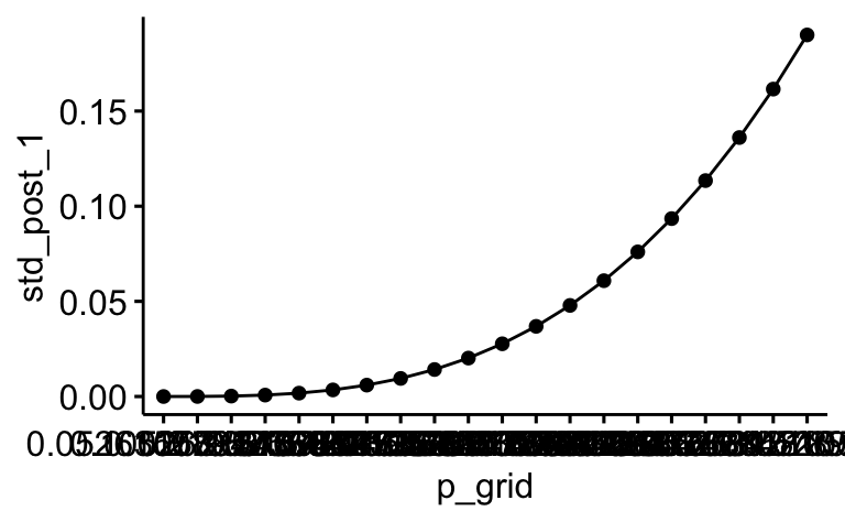

Oder mit ggplot2:

ggplot(dist) +
  aes(x = p_grid, y= std_post_1) +
  geom_line()+
  geom_point() +
  labs(x = "p(W)",
       y = "Posteriori-Wahrscheinlichkeit",
       title = "Daten: WWW")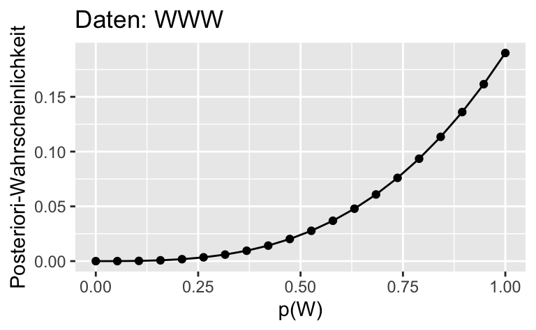

ggplot(dist) +
  aes(x = p_grid, y= std_post_2) +
  geom_line()+
  geom_point() +
  labs(x = "p(W)",
       y = "Posteriori-Wahrscheinlichkeit",
       title = "Daten: WWWL")

ggplot(dist) +
  aes(x = p_grid, y= std_post_3) +
  geom_line()+
  geom_point() +
  labs(x = "p(W)",
       y = "Posteriori-Wahrscheinlichkeit",
       title = "Daten: LWWLWWW")

---

Categories:

• probability
• bayes-grid
• rethink-chap2
• string