library(tidyverse)

dist <-
  tibble(
    # Gridwerte bestimmen:
    p_grid = seq(from = 0, to = 1, length.out = 21),
    # Priori-Wskt bestimmen:
    prior  = case_when(
      p_grid < 0.5 ~ 0,  # Null, wenn p < 0.5
      p_grid >= 0.5 ~ 1)) %>%  # 1, wenn p >= 0.5
  mutate(
    # Likelihood berechnen:
    likelihood_1 = dbinom(3, size = 3, prob = p_grid),
    likelihood_2 = dbinom(3, size = 4, prob = p_grid),
    likelihood_3 = dbinom(5, size = 7, prob = p_grid),
    # unstand. Posterior-Wskt:
    unstand_post_1 = likelihood_1 * prior,
    unstand_post_2 = likelihood_2 * prior,
    unstand_post_3 = likelihood_3 * prior,
    # stand. Post-Wskt:
    std_post_1 = unstand_post_1 / sum(unstand_post_1),
    std_post_2 = unstand_post_2 / sum(unstand_post_2),
    std_post_3 = unstand_post_3 / sum(unstand_post_3)
) Rethink2m2
probability
bayesbox
bayes
rethink-chap2
string
qm2
qm2-pruefung2023
Aufgabe
This question is taken from McElreath, R. (2020). Statistical rethinking: A Bayesian course with examples in R and Stan (2. Ed.). Taylor and Francis, CRC Press.
Recall the globe tossing model from the chapter (also see exercise globus1). Compute and plot the grid approximate posterior distribution for each of the following sets of observations. In each case, assume a uniform prior for p.
Data:
- WWW
- WWWL
- LWWLWWW
Now assume a prior for p that is equal to zero when p < 0.5 and is a positive constant when p ≥ 0.5. Again compute and plot the grid approximate posterior distribution for each of the sets of observations in the problem just above.
NB:
- Consider 21 different values for p such that
- Round to 2 decimal places.
Lösung
The solution is taken from this source.
Here is the Bayes Box:
| p_grid | prior | likelihood_1 | likelihood_2 | likelihood_3 | unstand_post_1 | unstand_post_2 | unstand_post_3 | std_post_1 | std_post_2 | std_post_3 |
|---|---|---|---|---|---|---|---|---|---|---|
| 0.00 | 0 | 0.00 | 0.00 | 0.00 | 0.00 | 0.00 | 0.00 | 0.00 | 0.00 | 0.00 |
| 0.05 | 0 | 0.00 | 0.00 | 0.00 | 0.00 | 0.00 | 0.00 | 0.00 | 0.00 | 0.00 |
| 0.10 | 0 | 0.00 | 0.00 | 0.00 | 0.00 | 0.00 | 0.00 | 0.00 | 0.00 | 0.00 |
| 0.15 | 0 | 0.00 | 0.01 | 0.00 | 0.00 | 0.00 | 0.00 | 0.00 | 0.00 | 0.00 |
| 0.20 | 0 | 0.01 | 0.03 | 0.00 | 0.00 | 0.00 | 0.00 | 0.00 | 0.00 | 0.00 |
| 0.25 | 0 | 0.02 | 0.05 | 0.01 | 0.00 | 0.00 | 0.00 | 0.00 | 0.00 | 0.00 |
| 0.30 | 0 | 0.03 | 0.08 | 0.03 | 0.00 | 0.00 | 0.00 | 0.00 | 0.00 | 0.00 |
| 0.35 | 0 | 0.04 | 0.11 | 0.05 | 0.00 | 0.00 | 0.00 | 0.00 | 0.00 | 0.00 |
| 0.40 | 0 | 0.06 | 0.15 | 0.08 | 0.00 | 0.00 | 0.00 | 0.00 | 0.00 | 0.00 |
| 0.45 | 0 | 0.09 | 0.20 | 0.12 | 0.00 | 0.00 | 0.00 | 0.00 | 0.00 | 0.00 |
| 0.50 | 1 | 0.13 | 0.25 | 0.16 | 0.13 | 0.25 | 0.16 | 0.02 | 0.07 | 0.07 |
| 0.55 | 1 | 0.17 | 0.30 | 0.21 | 0.17 | 0.30 | 0.21 | 0.03 | 0.09 | 0.10 |
| 0.60 | 1 | 0.22 | 0.35 | 0.26 | 0.22 | 0.35 | 0.26 | 0.04 | 0.10 | 0.12 |
| 0.65 | 1 | 0.27 | 0.38 | 0.30 | 0.27 | 0.38 | 0.30 | 0.05 | 0.11 | 0.13 |
| 0.70 | 1 | 0.34 | 0.41 | 0.32 | 0.34 | 0.41 | 0.32 | 0.07 | 0.12 | 0.14 |
| 0.75 | 1 | 0.42 | 0.42 | 0.31 | 0.42 | 0.42 | 0.31 | 0.08 | 0.13 | 0.14 |
| 0.80 | 1 | 0.51 | 0.41 | 0.28 | 0.51 | 0.41 | 0.28 | 0.10 | 0.12 | 0.12 |
| 0.85 | 1 | 0.61 | 0.37 | 0.21 | 0.61 | 0.37 | 0.21 | 0.12 | 0.11 | 0.09 |
| 0.90 | 1 | 0.73 | 0.29 | 0.12 | 0.73 | 0.29 | 0.12 | 0.14 | 0.09 | 0.06 |
| 0.95 | 1 | 0.86 | 0.17 | 0.04 | 0.86 | 0.17 | 0.04 | 0.16 | 0.05 | 0.02 |
| 1.00 | 1 | 1.00 | 0.00 | 0.00 | 1.00 | 0.00 | 0.00 | 0.19 | 0.00 | 0.00 |
Jetzt können wir das Diagramm zeichnen.
Mit ggpubr:
library(ggpubr)
ggline(dist,
       x = "p_grid",
       y = "std_post_1")
Oder mit ggplot2:
ggplot(dist) +
  aes(x = p_grid, y= std_post_1) +
  geom_line()+
  geom_point() +
  labs(x = "p(W)",
       y = "Posteriori-Wahrscheinlichkeit",
       title = "Daten: WWW")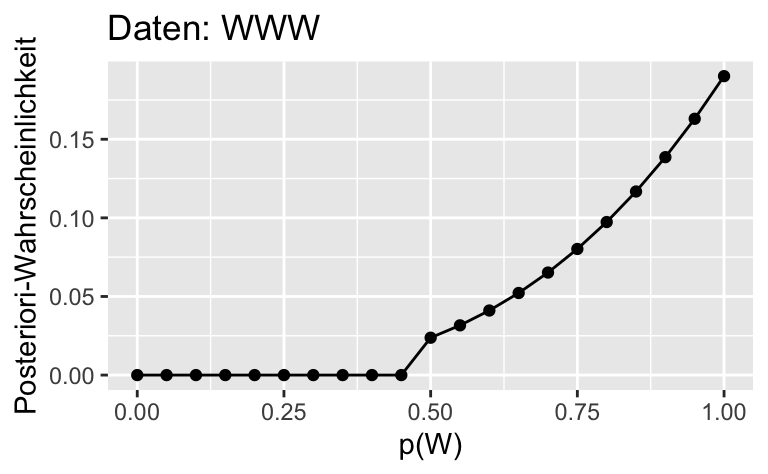
ggplot(dist) +
  aes(x = p_grid, y= std_post_2) +
  geom_line()+
  geom_point() +
  labs(x = "p(W)",
       y = "Posteriori-Wahrscheinlichkeit",
       title = "Daten: WWWL")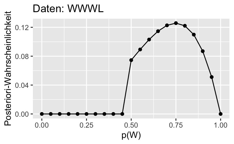
ggplot(dist) +
  aes(x = p_grid, y= std_post_3) +
  geom_line()+
  geom_point() +
  labs(x = "p(W)",
       y = "Posteriori-Wahrscheinlichkeit",
       title = "Daten: LWWLWWW")
Categories:
- probability
- bayesbox
- bayes
- rethink-chap2
- string